

 Set up docs MCP
ClickHouse はクエリを非常に高速に処理しますが、クエリ実行の仕組みはそれほど単純ではありません。SELECT クエリがどのように実行されるのかを見ていきましょう。これを説明するために、まず ClickHouse のテーブルにいくつかデータを追加してみます。
CREATE TABLE session_events(
   clientId UUID,
   sessionId UUID,
   pageId UUID,
   timestamp DateTime,
   type String
) ORDER BY (timestamp);

INSERT INTO session_events SELECT * FROM generateRandom('clientId UUID,
   sessionId UUID,
   pageId UUID,
   timestamp DateTime,
   type Enum(\'type1\', \'type2\')', 1, 10, 2) LIMIT 1000;
ClickHouse にデータが入ったので、いくつかのクエリを実行し、その実行の仕組みを見ていきましょう。クエリの実行はいくつもの段階に分解されます。クエリ実行の各段階は、対応する EXPLAIN クエリを使って分析し、トラブルシュートできます。これらの段階は以下の図にまとめられています。
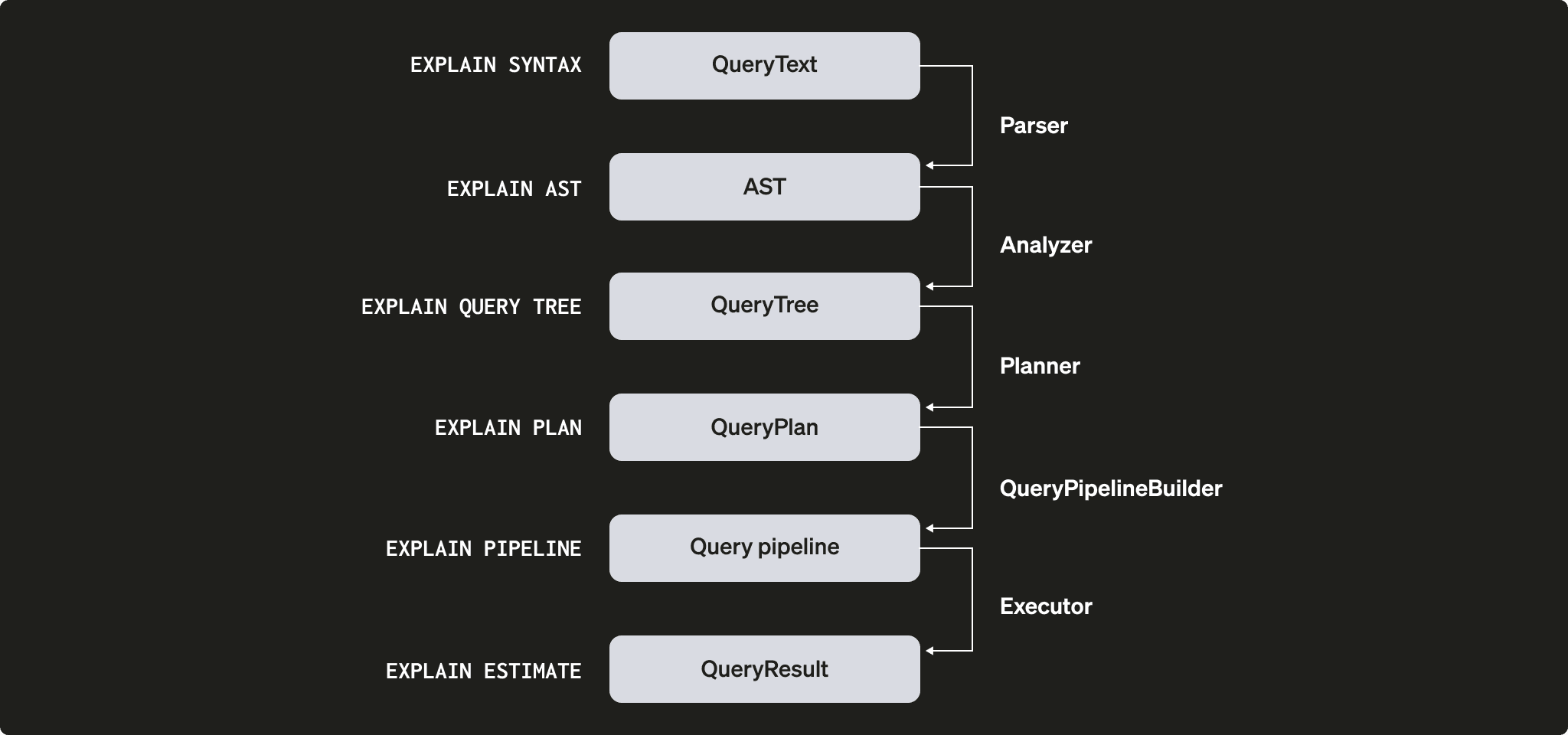
クエリ実行時に各要素がどのように機能するのかを見ていきましょう。いくつかのクエリを取り上げ、EXPLAIN ステートメントを使って確認します。
パーサー
パーサーの目的は、クエリテキストを AST (抽象構文木) へ変換することです。この処理は、EXPLAIN AST を使って可視化できます。
EXPLAIN AST SELECT min(timestamp) AS minimum_date, max(timestamp) AS maximum_date FROM session_events;┌─explain────────────────────────────────────────────┐
│ SelectWithUnionQuery (children 1) │
│ ExpressionList (children 1) │
│ SelectQuery (children 2) │
│ ExpressionList (children 2) │
│ Function min (alias minimum_date) (children 1) │
│ ExpressionList (children 1) │
│ Identifier timestamp │
│ Function max (alias maximum_date) (children 1) │
│ ExpressionList (children 1) │
│ Identifier timestamp │
│ TablesInSelectQuery (children 1) │
│ TablesInSelectQueryElement (children 1) │
│ TableExpression (children 1) │
│ TableIdentifier session_events │
└────────────────────────────────────────────────────┘出力は抽象構文木 (AST) で、以下のように可視化できます。
graph TD
    swuq["SelectWithUnionQuery"] --> el_root["ExpressionList"]
    el_root --> sq["SelectQuery"]
    sq --> el_select["ExpressionList"]
    sq --> tisq["TablesInSelectQuery"]
    el_select --> fmin["Function min (alias minimum_date)"]
    el_select --> fmax["Function max (alias maximum_date)"]
    fmin --> el_min["ExpressionList"]
    el_min --> id_min["Identifier timestamp"]
    fmax --> el_max["ExpressionList"]
    el_max --> id_max["Identifier timestamp"]
    tisq --> tisqe["TablesInSelectQueryElement"]
    tisqe --> te["TableExpression"]
    te --> ti["TableIdentifier session_events"]
各ノードには対応する子ノードがあり、木全体でクエリ全体の構造を表しています。これはクエリを処理するための論理構造です。エンドユーザーの観点では (クエリ実行に関心がある場合を除き) 、それほど有用ではありません。このツールは主に開発者が使用します。
アナライザ
ClickHouse には現在、アナライザに 2 つのアーキテクチャがあります。古いアーキテクチャは、enable_analyzer=0 を設定することで使用できます。現在のアーキテクチャは、ClickHouse 24.3 以降デフォルトで有効になっています。古いものは非推奨であり、後方互換性のためだけに維持されているため、ここでは現在のアーキテクチャについてのみ説明します。
アナライザは、クエリ実行における重要な段階です。AST を受け取り、それをクエリツリーに変換します。AST に対するクエリツリーの主な利点は、たとえばストレージのように、多くの部分が解決済みになることです。どのテーブルから読み取るかも分かり、別名も解決され、ツリーは使われているさまざまなデータ型も把握します。こうした利点により、アナライザは最適化を適用できます。これらの最適化は「パス」を通じて行われます。各パスは異なる最適化を探します。すべてのパスは こちら で確認できます。では、前のクエリを使って実際に見てみましょう。
EXPLAIN QUERY TREE passes=0 SELECT min(timestamp) AS minimum_date, max(timestamp) AS maximum_date FROM session_events SETTINGS allow_experimental_analyzer=1;┌─explain────────────────────────────────────────────────────────────────────────────────┐
│ QUERY id: 0 │
│ PROJECTION │
│ LIST id: 1, nodes: 2 │
│ FUNCTION id: 2, alias: minimum_date, function_name: min, function_type: ordinary │
│ ARGUMENTS │
│ LIST id: 3, nodes: 1 │
│ IDENTIFIER id: 4, identifier: timestamp │
│ FUNCTION id: 5, alias: maximum_date, function_name: max, function_type: ordinary │
│ ARGUMENTS │
│ LIST id: 6, nodes: 1 │
│ IDENTIFIER id: 7, identifier: timestamp │
│ JOIN TREE │
│ IDENTIFIER id: 8, identifier: session_events │
│ SETTINGS allow_experimental_analyzer=1 │
└────────────────────────────────────────────────────────────────────────────────────────┘EXPLAIN QUERY TREE passes=20 SELECT min(timestamp) AS minimum_date, max(timestamp) AS maximum_date FROM session_events SETTINGS allow_experimental_analyzer=1;┌─explain───────────────────────────────────────────────────────────────────────────────────┐
│ QUERY id: 0 │
│ PROJECTION COLUMNS │
│ minimum_date DateTime │
│ maximum_date DateTime │
│ PROJECTION │
│ LIST id: 1, nodes: 2 │
│ FUNCTION id: 2, function_name: min, function_type: aggregate, result_type: DateTime │
│ ARGUMENTS │
│ LIST id: 3, nodes: 1 │
│ COLUMN id: 4, column_name: timestamp, result_type: DateTime, source_id: 5 │
│ FUNCTION id: 6, function_name: max, function_type: aggregate, result_type: DateTime │
│ ARGUMENTS │
│ LIST id: 7, nodes: 1 │
│ COLUMN id: 4, column_name: timestamp, result_type: DateTime, source_id: 5 │
│ JOIN TREE │
│ TABLE id: 5, alias: __table1, table_name: default.session_events │
│ SETTINGS allow_experimental_analyzer=1 │
└───────────────────────────────────────────────────────────────────────────────────────────┘2回の実行を比較すると、別名とPROJECTIONの解決を確認できます。
プランナー
プランナーはクエリツリーを受け取り、それを基にクエリプランを構築します。クエリツリーは特定のクエリで何を行いたいかを示し、クエリプランはそれをどのように実行するかを示します。追加の最適化もクエリプランの一部として行われます。クエリプランを確認するには、EXPLAIN PLAN または EXPLAIN を使用できます (EXPLAIN は EXPLAIN PLAN を実行します) 。
EXPLAIN PLAN WITH
   (
       SELECT count(*)
       FROM session_events
   ) AS total_rows
SELECT type, min(timestamp) AS minimum_date, max(timestamp) AS maximum_date, count(*) /total_rows * 100 AS percentage FROM session_events GROUP BY type
┌─explain──────────────────────────────────────────┐
│ Expression ((Projection + Before ORDER BY)) │
│ Aggregating │
│ Expression (Before GROUP BY) │
│ ReadFromMergeTree (default.session_events) │
└──────────────────────────────────────────────────┘これでもある程度の情報は得られますが、さらに詳しい情報を取得できます。たとえば、どのカラムに対してPROJECTIONが必要なのか、そのカラム名を知りたい場合があります。ヘッダーをクエリに追加できます。
EXPLAIN header = 1
WITH (
       SELECT count(*)
       FROM session_events
   ) AS total_rows
SELECT
   type,
   min(timestamp) AS minimum_date,
   max(timestamp) AS maximum_date,
   (count(*) / total_rows) * 100 AS percentage
FROM session_events
GROUP BY type
┌─explain──────────────────────────────────────────┐
│ Expression ((Projection + Before ORDER BY)) │
│ Header: type String │
│ minimum_date DateTime │
│ maximum_date DateTime │
│ percentage Nullable(Float64) │
│ Aggregating │
│ Header: type String │
│ min(timestamp) DateTime │
│ max(timestamp) DateTime │
│ count() UInt64 │
│ Expression (Before GROUP BY) │
│ Header: timestamp DateTime │
│ type String │
│ ReadFromMergeTree (default.session_events) │
│ Header: timestamp DateTime │
│ type String │
└──────────────────────────────────────────────────┘これで、最後の PROJECTION に対して作成する必要があるカラム名 (minimum_date、maximum_date、percentage) はわかりましたが、実行する必要があるすべての actions の詳細も確認したいことがあるでしょう。その場合は、actions=1 を設定します。
EXPLAIN actions = 1
WITH (
       SELECT count(*)
       FROM session_events
   ) AS total_rows
SELECT
   type,
   min(timestamp) AS minimum_date,
   max(timestamp) AS maximum_date,
   (count(*) / total_rows) * 100 AS percentage
FROM session_events
GROUP BY type
┌─explain────────────────────────────────────────────────────────────────────────────────────────────────────────────────────────────────────┐
│ Expression ((Projection + Before ORDER BY)) │
│ Actions: INPUT :: 0 -> type String : 0 │
│ INPUT : 1 -> min(timestamp) DateTime : 1 │
│ INPUT : 2 -> max(timestamp) DateTime : 2 │
│ INPUT : 3 -> count() UInt64 : 3 │
│ COLUMN Const(Nullable(UInt64)) -> total_rows Nullable(UInt64) : 4 │
│ COLUMN Const(UInt8) -> 100 UInt8 : 5 │
│ ALIAS min(timestamp) :: 1 -> minimum_date DateTime : 6 │
│ ALIAS max(timestamp) :: 2 -> maximum_date DateTime : 1 │
│ FUNCTION divide(count() :: 3, total_rows :: 4) -> divide(count(), total_rows) Nullable(Float64) : 2 │
│ FUNCTION multiply(divide(count(), total_rows) :: 2, 100 :: 5) -> multiply(divide(count(), total_rows), 100) Nullable(Float64) : 4 │
│ ALIAS multiply(divide(count(), total_rows), 100) :: 4 -> percentage Nullable(Float64) : 5 │
│ Positions: 0 6 1 5 │
│ Aggregating │
│ Keys: type │
│ Aggregates: │
│ min(timestamp) │
│ Function: min(DateTime) → DateTime │
│ Arguments: timestamp │
│ max(timestamp) │
│ Function: max(DateTime) → DateTime │
│ Arguments: timestamp │
│ count() │
│ Function: count() → UInt64 │
│ Arguments: none │
│ Skip merging: 0 │
│ Expression (Before GROUP BY) │
│ Actions: INPUT :: 0 -> timestamp DateTime : 0 │
│ INPUT :: 1 -> type String : 1 │
│ Positions: 0 1 │
│ ReadFromMergeTree (default.session_events) │
│ ReadType: Default │
│ Parts: 1 │
│ Granules: 1 │
└────────────────────────────────────────────────────────────────────────────────────────────────────────────────────────────────────────────┘これで、使用されているすべての入力、関数、別名、データ型を確認できます。プランナーが適用する最適化の一部は、こちらで確認できます。
クエリパイプライン
クエリパイプラインはクエリプランから生成されます。クエリパイプラインはクエリプランと非常に似ていますが、ツリーではなくグラフである点が異なります。ClickHouse がクエリをどのように実行するか、またどのリソースが使用されるかを把握できます。クエリパイプラインを分析することで、入出力のどこにボトルネックがあるかを特定できます。前述のクエリを使って、クエリパイプラインの実行を確認してみましょう。
EXPLAIN PIPELINE
WITH (
       SELECT count(*)
       FROM session_events
   ) AS total_rows
SELECT
   type,
   min(timestamp) AS minimum_date,
   max(timestamp) AS maximum_date,
   (count(*) / total_rows) * 100 AS percentage
FROM session_events
GROUP BY type;
┌─explain────────────────────────────────────────────────────────────────────┐
│ (Expression) │
│ ExpressionTransform × 2 │
│ (Aggregating) │
│ Resize 1 → 2 │
│ AggregatingTransform │
│ (Expression) │
│ ExpressionTransform │
│ (ReadFromMergeTree) │
│ MergeTreeSelect(pool: PrefetchedReadPool, algorithm: Thread) 0 → 1 │
└────────────────────────────────────────────────────────────────────────────┘括弧内はクエリプランのステップ、その隣はプロセッサです。有益な情報ですが、グラフ構造であるため、視覚的に表示できると便利です。graph 設定を 1 に設定し、出力フォーマットを TSV に指定することができます:
EXPLAIN PIPELINE graph=1 WITH
   (
       SELECT count(*)
       FROM session_events
   ) AS total_rows
SELECT type, min(timestamp) AS minimum_date, max(timestamp) AS maximum_date, count(*) /total_rows * 100 AS percentage FROM session_events GROUP BY type FORMAT TSV;
digraph
{
rankdir="LR";
{ node [shape = rect]
subgraph cluster_0 {
label ="Expression";
style=filled;
color=lightgrey;
node [style=filled,color=white];
{ rank = same;
n5 [label="ExpressionTransform × 2"];
}
}
subgraph cluster_1 {
label ="Aggregating";
style=filled;
color=lightgrey;
node [style=filled,color=white];
{ rank = same;
n3 [label="AggregatingTransform"];
n4 [label="Resize"];
}
}
subgraph cluster_2 {
label ="Expression";
style=filled;
color=lightgrey;
node [style=filled,color=white];
{ rank = same;
n2 [label="ExpressionTransform"];
}
}
subgraph cluster_3 {
label ="ReadFromMergeTree";
style=filled;
color=lightgrey;
node [style=filled,color=white];
{ rank = same;
n1 [label="MergeTreeSelect(pool: PrefetchedReadPool, algorithm: Thread)"];
}
}
}
n3 -> n4 [label=""];
n4 -> n5 [label="× 2"];
n2 -> n3 [label=""];
n1 -> n2 [label=""];
}この出力をコピーしてこちらに貼り付けると、以下のグラフが生成されます。
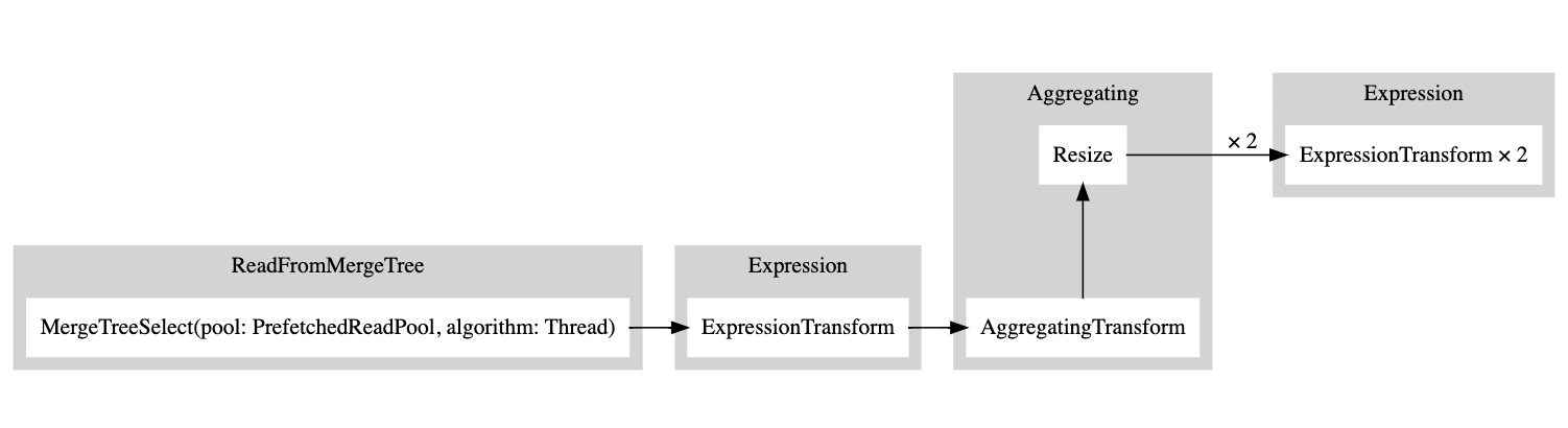
白い長方形はパイプラインノードを、灰色の長方形はクエリプランのステップを表し、x に続く数字は使用されている入力/出力の数を示します。コンパクト形式での表示が不要な場合は、compact=0 を追加してください:
EXPLAIN PIPELINE graph = 1, compact = 0
WITH (
       SELECT count(*)
       FROM session_events
   ) AS total_rows
SELECT
   type,
   min(timestamp) AS minimum_date,
   max(timestamp) AS maximum_date,
   (count(*) / total_rows) * 100 AS percentage
FROM session_events
GROUP BY type
FORMAT TSV
digraph
{
rankdir="LR";
{ node [shape = rect]
n0[label="MergeTreeSelect(pool: PrefetchedReadPool, algorithm: Thread)"];
n1[label="ExpressionTransform"];
n2[label="AggregatingTransform"];
n3[label="Resize"];
n4[label="ExpressionTransform"];
n5[label="ExpressionTransform"];
}
n0 -> n1;
n1 -> n2;
n2 -> n3;
n3 -> n4;
n3 -> n5;
}
ClickHouse はなぜ複数のスレッドでテーブルを読み込まないのでしょうか。テーブルにさらにデータを追加してみましょう:
INSERT INTO session_events SELECT * FROM generateRandom('clientId UUID,
   sessionId UUID,
   pageId UUID,
   timestamp DateTime,
type Enum(\'type1\', \'type2\')', 1, 10, 2) LIMIT 1000000;それでは、EXPLAIN クエリをもう一度実行してみましょう。
EXPLAIN PIPELINE graph = 1, compact = 0
WITH (
       SELECT count(*)
       FROM session_events
   ) AS total_rows
SELECT
   type,
   min(timestamp) AS minimum_date,
   max(timestamp) AS maximum_date,
   (count(*) / total_rows) * 100 AS percentage
FROM session_events
GROUP BY type
FORMAT TSV
digraph
{
rankdir="LR";
{ node [shape = rect]
n0[label="MergeTreeSelect(pool: PrefetchedReadPool, algorithm: Thread)"];
n1[label="MergeTreeSelect(pool: PrefetchedReadPool, algorithm: Thread)"];
n2[label="ExpressionTransform"];
n3[label="ExpressionTransform"];
n4[label="StrictResize"];
n5[label="AggregatingTransform"];
n6[label="AggregatingTransform"];
n7[label="Resize"];
n8[label="ExpressionTransform"];
n9[label="ExpressionTransform"];
}
n0 -> n2;
n1 -> n3;
n2 -> n4;
n3 -> n4;
n4 -> n5;
n4 -> n6;
n5 -> n7;
n6 -> n7;
n7 -> n8;
n7 -> n9;
}
つまり、データ量が十分でなかったため、エグゼキュータは処理を並列化しないと判断しました。さらに行を追加すると、グラフに示されているように、エグゼキュータは複数のスレッドを使用するようになりました。
エグゼキュータ
最後に、クエリ実行の最終段階はエグゼキュータが担います。エグゼキュータはクエリパイプラインを受け取り、実行します。SELECT、INSERT、INSERT SELECT のどれを実行するかによって、使用されるエグゼキュータの種類は異なります。