

 Set up docs MCP
ClickHouse 处理查询的速度极快,但查询的执行过程并不简单。下面我们来了解一下 SELECT 查询是如何执行的。为了便于说明,先在 ClickHouse 的一个表中添加一些数据:
CREATE TABLE session_events(
   clientId UUID,
   sessionId UUID,
   pageId UUID,
   timestamp DateTime,
   type String
) ORDER BY (timestamp);

INSERT INTO session_events SELECT * FROM generateRandom('clientId UUID,
   sessionId UUID,
   pageId UUID,
   timestamp DateTime,
   type Enum(\'type1\', \'type2\')', 1, 10, 2) LIMIT 1000;
现在 ClickHouse 中已经有了一些数据,我们可以运行一些查询并了解它们的执行过程。查询执行会被拆分为多个步骤。查询执行的每个步骤都可以通过相应的 EXPLAIN 查询进行分析和故障排查。下图概括了这些步骤:
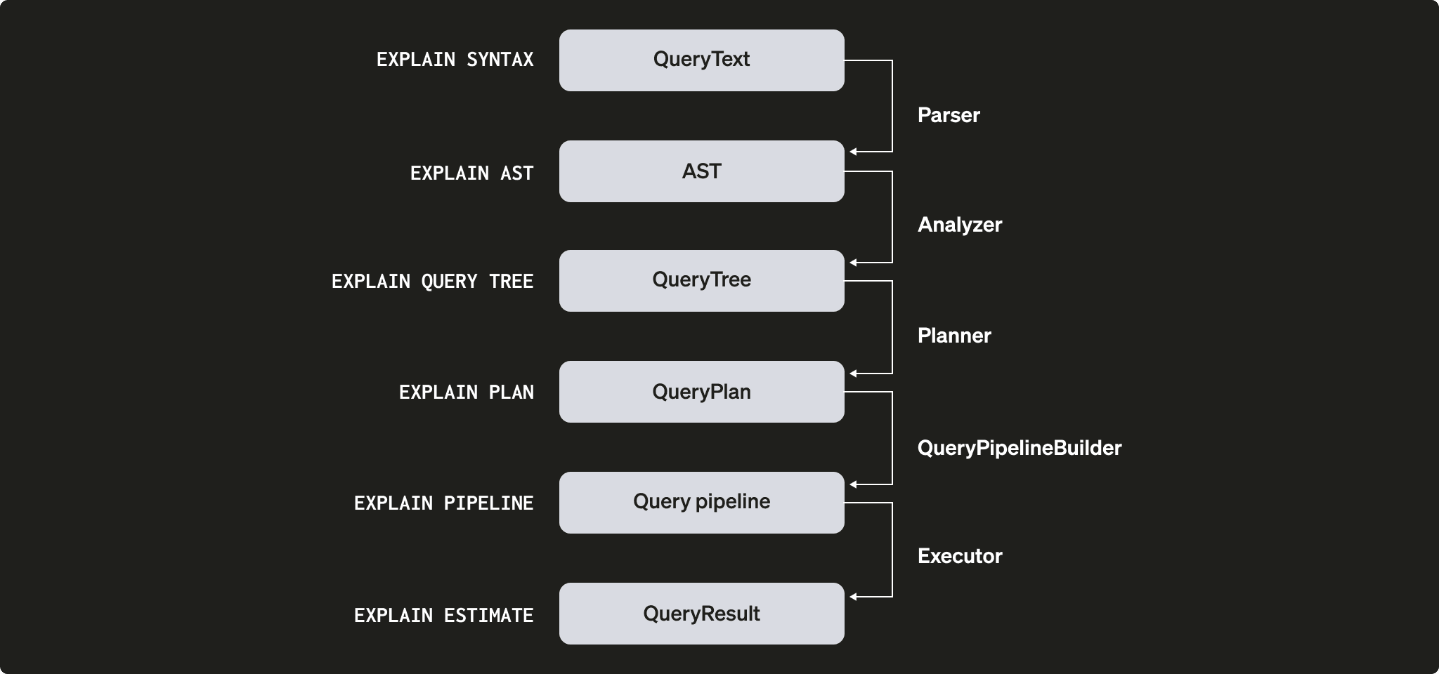
下面我们来看这些环节在查询执行过程中是如何工作的。我们将选取几个查询,然后使用 EXPLAIN 语句来分析它们。
解析器
解析器的目标是将查询文本转换为 AST (抽象语法树) 。可以用 EXPLAIN AST 直观地展示这一步骤:
EXPLAIN AST SELECT min(timestamp) AS minimum_date, max(timestamp) AS maximum_date FROM session_events;┌─explain────────────────────────────────────────────┐
│ SelectWithUnionQuery (children 1) │
│ ExpressionList (children 1) │
│ SelectQuery (children 2) │
│ ExpressionList (children 2) │
│ Function min (alias minimum_date) (children 1) │
│ ExpressionList (children 1) │
│ Identifier timestamp │
│ Function max (alias maximum_date) (children 1) │
│ ExpressionList (children 1) │
│ Identifier timestamp │
│ TablesInSelectQuery (children 1) │
│ TablesInSelectQueryElement (children 1) │
│ TableExpression (children 1) │
│ TableIdentifier session_events │
└────────────────────────────────────────────────────┘输出结果是一棵抽象语法树,可视化效果如下所示:
graph TD
    swuq["SelectWithUnionQuery"] --> el_root["ExpressionList"]
    el_root --> sq["SelectQuery"]
    sq --> el_select["ExpressionList"]
    sq --> tisq["TablesInSelectQuery"]
    el_select --> fmin["Function min (alias minimum_date)"]
    el_select --> fmax["Function max (alias maximum_date)"]
    fmin --> el_min["ExpressionList"]
    el_min --> id_min["Identifier timestamp"]
    fmax --> el_max["ExpressionList"]
    el_max --> id_max["Identifier timestamp"]
    tisq --> tisqe["TablesInSelectQueryElement"]
    tisqe --> te["TableExpression"]
    te --> ti["TableIdentifier session_events"]
每个节点都有对应的子节点,整棵树表示查询的整体结构。这是一种有助于处理查询的逻辑结构。从终端用户的角度来看 (除非你对查询执行感兴趣) ,它的实用性并不高;这个工具主要供开发者使用。
Analyzer
ClickHouse 目前有两套 Analyzer 架构。你可以通过设置 enable_analyzer=0 使用旧架构。自 ClickHouse 24.3 起,当前架构已默认启用。由于旧架构已被弃用并且仅为向后兼容而保留,这里我们只介绍当前架构。
analyzer 是查询执行中的一个重要步骤。它接收 AST,并将其转换为查询树。与 AST 相比,查询树的主要优势在于其中许多组成部分都已完成解析,例如具体使用的存储。我们还能够确定应从哪张表读取数据,别名也会被解析,并且查询树也知道所使用的各种数据类型。有了这些优势,analyzer 就可以应用优化。这些优化是通过“passes”实现的。每个 pass 都会寻找不同的优化机会。你可以在这里查看所有 passes,下面我们结合之前的查询来看实际效果:
EXPLAIN QUERY TREE passes=0 SELECT min(timestamp) AS minimum_date, max(timestamp) AS maximum_date FROM session_events SETTINGS allow_experimental_analyzer=1;┌─explain────────────────────────────────────────────────────────────────────────────────┐
│ QUERY id: 0 │
│ PROJECTION │
│ LIST id: 1, nodes: 2 │
│ FUNCTION id: 2, alias: minimum_date, function_name: min, function_type: ordinary │
│ ARGUMENTS │
│ LIST id: 3, nodes: 1 │
│ IDENTIFIER id: 4, identifier: timestamp │
│ FUNCTION id: 5, alias: maximum_date, function_name: max, function_type: ordinary │
│ ARGUMENTS │
│ LIST id: 6, nodes: 1 │
│ IDENTIFIER id: 7, identifier: timestamp │
│ JOIN TREE │
│ IDENTIFIER id: 8, identifier: session_events │
│ SETTINGS allow_experimental_analyzer=1 │
└────────────────────────────────────────────────────────────────────────────────────────┘EXPLAIN QUERY TREE passes=20 SELECT min(timestamp) AS minimum_date, max(timestamp) AS maximum_date FROM session_events SETTINGS allow_experimental_analyzer=1;┌─explain───────────────────────────────────────────────────────────────────────────────────┐
│ QUERY id: 0 │
│ PROJECTION COLUMNS │
│ minimum_date DateTime │
│ maximum_date DateTime │
│ PROJECTION │
│ LIST id: 1, nodes: 2 │
│ FUNCTION id: 2, function_name: min, function_type: aggregate, result_type: DateTime │
│ ARGUMENTS │
│ LIST id: 3, nodes: 1 │
│ COLUMN id: 4, column_name: timestamp, result_type: DateTime, source_id: 5 │
│ FUNCTION id: 6, function_name: max, function_type: aggregate, result_type: DateTime │
│ ARGUMENTS │
│ LIST id: 7, nodes: 1 │
│ COLUMN id: 4, column_name: timestamp, result_type: DateTime, source_id: 5 │
│ JOIN TREE │
│ TABLE id: 5, alias: __table1, table_name: default.session_events │
│ SETTINGS allow_experimental_analyzer=1 │
└───────────────────────────────────────────────────────────────────────────────────────────┘对比这两次执行结果,可以看到别名和投影的解析过程。
规划器
规划器接收查询树,并据此生成查询计划。查询树描述的是我们希望对某个特定查询执行什么操作,而查询计划说明的是这些操作将如何执行。进一步的优化也会在生成查询计划的过程中完成。你可以使用 EXPLAIN PLAN 或 EXPLAIN 来查看查询计划 (EXPLAIN 会执行 EXPLAIN PLAN) 。
EXPLAIN PLAN WITH
   (
       SELECT count(*)
       FROM session_events
   ) AS total_rows
SELECT type, min(timestamp) AS minimum_date, max(timestamp) AS maximum_date, count(*) /total_rows * 100 AS percentage FROM session_events GROUP BY type
┌─explain──────────────────────────────────────────┐
│ Expression ((Projection + Before ORDER BY)) │
│ Aggregating │
│ Expression (Before GROUP BY) │
│ ReadFromMergeTree (default.session_events) │
└──────────────────────────────────────────────────┘虽然这已经给了我们一些信息,但我们还能获取更多。例如,我们可能还想知道需要在其上创建投影的列名。你可以在查询中添加请求头:
EXPLAIN header = 1
WITH (
       SELECT count(*)
       FROM session_events
   ) AS total_rows
SELECT
   type,
   min(timestamp) AS minimum_date,
   max(timestamp) AS maximum_date,
   (count(*) / total_rows) * 100 AS percentage
FROM session_events
GROUP BY type
┌─explain──────────────────────────────────────────┐
│ Expression ((Projection + Before ORDER BY)) │
│ Header: type String │
│ minimum_date DateTime │
│ maximum_date DateTime │
│ percentage Nullable(Float64) │
│ Aggregating │
│ Header: type String │
│ min(timestamp) DateTime │
│ max(timestamp) DateTime │
│ count() UInt64 │
│ Expression (Before GROUP BY) │
│ Header: timestamp DateTime │
│ type String │
│ ReadFromMergeTree (default.session_events) │
│ Header: timestamp DateTime │
│ type String │
└──────────────────────────────────────────────────┘现在你已经知道了最后一个 Projection 需要创建哪些列名 (minimum_date、maximum_date 和 percentage) ,但你可能还想查看所有待执行操作的详细信息。你可以通过设置 actions=1 来实现。
EXPLAIN actions = 1
WITH (
       SELECT count(*)
       FROM session_events
   ) AS total_rows
SELECT
   type,
   min(timestamp) AS minimum_date,
   max(timestamp) AS maximum_date,
   (count(*) / total_rows) * 100 AS percentage
FROM session_events
GROUP BY type
┌─explain────────────────────────────────────────────────────────────────────────────────────────────────────────────────────────────────────┐
│ Expression ((Projection + Before ORDER BY)) │
│ Actions: INPUT :: 0 -> type String : 0 │
│ INPUT : 1 -> min(timestamp) DateTime : 1 │
│ INPUT : 2 -> max(timestamp) DateTime : 2 │
│ INPUT : 3 -> count() UInt64 : 3 │
│ COLUMN Const(Nullable(UInt64)) -> total_rows Nullable(UInt64) : 4 │
│ COLUMN Const(UInt8) -> 100 UInt8 : 5 │
│ ALIAS min(timestamp) :: 1 -> minimum_date DateTime : 6 │
│ ALIAS max(timestamp) :: 2 -> maximum_date DateTime : 1 │
│ FUNCTION divide(count() :: 3, total_rows :: 4) -> divide(count(), total_rows) Nullable(Float64) : 2 │
│ FUNCTION multiply(divide(count(), total_rows) :: 2, 100 :: 5) -> multiply(divide(count(), total_rows), 100) Nullable(Float64) : 4 │
│ ALIAS multiply(divide(count(), total_rows), 100) :: 4 -> percentage Nullable(Float64) : 5 │
│ Positions: 0 6 1 5 │
│ Aggregating │
│ Keys: type │
│ Aggregates: │
│ min(timestamp) │
│ Function: min(DateTime) → DateTime │
│ Arguments: timestamp │
│ max(timestamp) │
│ Function: max(DateTime) → DateTime │
│ Arguments: timestamp │
│ count() │
│ Function: count() → UInt64 │
│ Arguments: none │
│ Skip merging: 0 │
│ Expression (Before GROUP BY) │
│ Actions: INPUT :: 0 -> timestamp DateTime : 0 │
│ INPUT :: 1 -> type String : 1 │
│ Positions: 0 1 │
│ ReadFromMergeTree (default.session_events) │
│ ReadType: Default │
│ Parts: 1 │
│ Granules: 1 │
└────────────────────────────────────────────────────────────────────────────────────────────────────────────────────────────────────────────┘现在,你可以看到所有正在使用的输入、函数、别名和数据类型。你还可以在这里查看规划器将应用的部分优化。
查询管道
查询管道由查询计划生成。查询管道与查询计划非常相似,区别在于它不是树形结构,而是图结构。它展示了 ClickHouse 将如何执行查询以及将使用哪些资源。分析查询管道对于定位输入/输出方面的性能瓶颈非常有帮助。下面以之前的查询为例,来看看查询管道的执行情况:
EXPLAIN PIPELINE
WITH (
       SELECT count(*)
       FROM session_events
   ) AS total_rows
SELECT
   type,
   min(timestamp) AS minimum_date,
   max(timestamp) AS maximum_date,
   (count(*) / total_rows) * 100 AS percentage
FROM session_events
GROUP BY type;
┌─explain────────────────────────────────────────────────────────────────────┐
│ (Expression) │
│ ExpressionTransform × 2 │
│ (Aggregating) │
│ Resize 1 → 2 │
│ AggregatingTransform │
│ (Expression) │
│ ExpressionTransform │
│ (ReadFromMergeTree) │
│ MergeTreeSelect(pool: PrefetchedReadPool, algorithm: Thread) 0 → 1 │
└────────────────────────────────────────────────────────────────────────────┘括号内是查询计划步骤,旁边是处理器。这些信息非常有用,但由于这本质上是一个图结构,如果能将其可视化会更加直观。我们可以将 graph 设置为 1,并将输出格式指定为 TSV:
EXPLAIN PIPELINE graph=1 WITH
   (
       SELECT count(*)
       FROM session_events
   ) AS total_rows
SELECT type, min(timestamp) AS minimum_date, max(timestamp) AS maximum_date, count(*) /total_rows * 100 AS percentage FROM session_events GROUP BY type FORMAT TSV;
digraph
{
rankdir="LR";
{ node [shape = rect]
subgraph cluster_0 {
label ="Expression";
style=filled;
color=lightgrey;
node [style=filled,color=white];
{ rank = same;
n5 [label="ExpressionTransform × 2"];
}
}
subgraph cluster_1 {
label ="Aggregating";
style=filled;
color=lightgrey;
node [style=filled,color=white];
{ rank = same;
n3 [label="AggregatingTransform"];
n4 [label="Resize"];
}
}
subgraph cluster_2 {
label ="Expression";
style=filled;
color=lightgrey;
node [style=filled,color=white];
{ rank = same;
n2 [label="ExpressionTransform"];
}
}
subgraph cluster_3 {
label ="ReadFromMergeTree";
style=filled;
color=lightgrey;
node [style=filled,color=white];
{ rank = same;
n1 [label="MergeTreeSelect(pool: PrefetchedReadPool, algorithm: Thread)"];
}
}
}
n3 -> n4 [label=""];
n4 -> n5 [label="× 2"];
n2 -> n3 [label=""];
n1 -> n2 [label=""];
}您可以将此输出复制并粘贴到此处,从而生成以下图形:
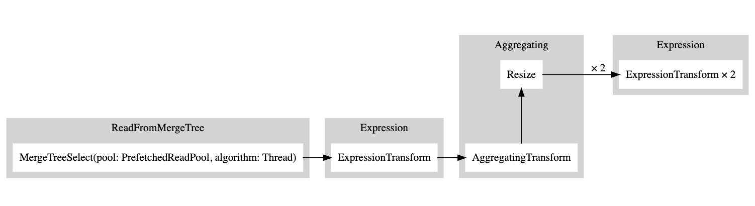
白色矩形对应管道节点,灰色矩形对应查询计划步骤,x 后跟的数字表示当前使用的输入/输出数量。如果不希望以紧凑形式显示,可以添加 compact=0:
EXPLAIN PIPELINE graph = 1, compact = 0
WITH (
       SELECT count(*)
       FROM session_events
   ) AS total_rows
SELECT
   type,
   min(timestamp) AS minimum_date,
   max(timestamp) AS maximum_date,
   (count(*) / total_rows) * 100 AS percentage
FROM session_events
GROUP BY type
FORMAT TSV
digraph
{
rankdir="LR";
{ node [shape = rect]
n0[label="MergeTreeSelect(pool: PrefetchedReadPool, algorithm: Thread)"];
n1[label="ExpressionTransform"];
n2[label="AggregatingTransform"];
n3[label="Resize"];
n4[label="ExpressionTransform"];
n5[label="ExpressionTransform"];
}
n0 -> n1;
n1 -> n2;
n2 -> n3;
n3 -> n4;
n3 -> n5;
}
为什么 ClickHouse 没有使用多个线程从表中读取数据?我们来尝试向表中添加更多数据:
INSERT INTO session_events SELECT * FROM generateRandom('clientId UUID,
   sessionId UUID,
   pageId UUID,
   timestamp DateTime,
   type Enum(\'type1\', \'type2\')', 1, 10, 2) LIMIT 1000000;
现在再次运行我们的 EXPLAIN 查询:
EXPLAIN PIPELINE graph = 1, compact = 0
WITH (
       SELECT count(*)
       FROM session_events
   ) AS total_rows
SELECT
   type,
   min(timestamp) AS minimum_date,
   max(timestamp) AS maximum_date,
   (count(*) / total_rows) * 100 AS percentage
FROM session_events
GROUP BY type
FORMAT TSV
digraph
{
rankdir="LR";
{ node [shape = rect]
n0[label="MergeTreeSelect(pool: PrefetchedReadPool, algorithm: Thread)"];
n1[label="MergeTreeSelect(pool: PrefetchedReadPool, algorithm: Thread)"];
n2[label="ExpressionTransform"];
n3[label="ExpressionTransform"];
n4[label="StrictResize"];
n5[label="AggregatingTransform"];
n6[label="AggregatingTransform"];
n7[label="Resize"];
n8[label="ExpressionTransform"];
n9[label="ExpressionTransform"];
}
n0 -> n2;
n1 -> n3;
n2 -> n4;
n3 -> n4;
n4 -> n5;
n4 -> n6;
n5 -> n7;
n6 -> n7;
n7 -> n8;
n7 -> n9;
}
因此,执行器认为无需将这些操作并行化,因为数据量还不够大。增加更多行后,执行器便决定改用多个线程,如图所示。
执行器
最后,查询执行的最终一步由执行器完成。它会接收查询管道并执行。根据执行的是 SELECT、INSERT 还是 INSERT SELECT,所使用的执行器类型也会不同。